DECISION TREES
OVERVIEW
Decision Trees are a popular supervised learning algorithm used for both classification and regression tasks in machine learning. They recursively partition the feature space into smaller regions based on feature values, ultimately resulting in a tree-like structure. It requires labeled data.
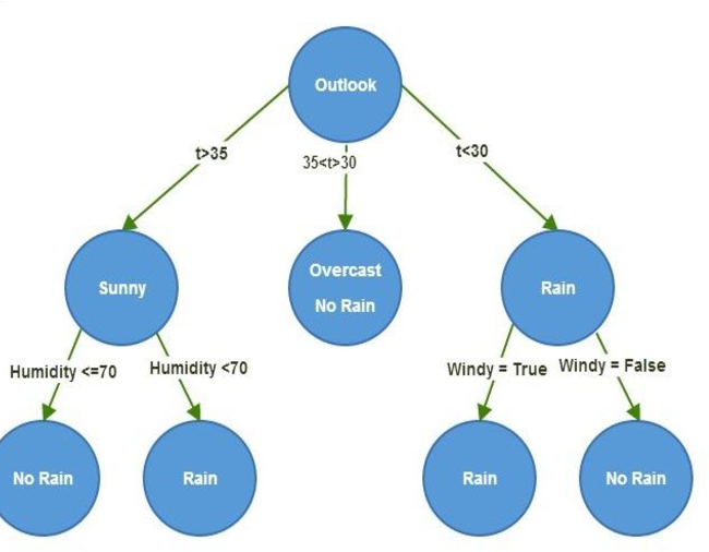
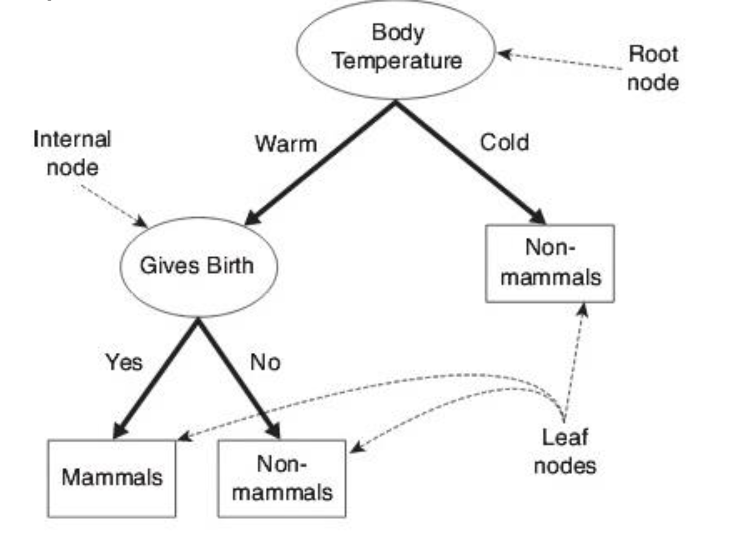
The tree has:
- Root Node: No incoming edges and zero or more outgoing edges. It contains attribute test condition(s). It is an impure node.
- Internal Node: Exactly ONE incoming edge and TWO or more outgoing. It contains attribute test condition(s). It is an impure node.
- Leaf/Terminal Node: ONE incoming, no outgoing. Each leaf node is assigned a class label. It is a pure node i.e, no impurity.
Building Decision Trees:
There are an infinite number of possible decision trees that can be constructed from a set of features as we can start with any feature as the root node.
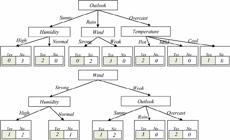
Finding the optimal tree is an intractable problem as the search space is exponential. Algorithms can find “good” decision trees using the Greedy Top-Down approach they make a series of locally optimal decisions.
Example: Hunt's Algorithm
Hunt's is the basis of ID3, C4.5, and CART
Metrics Used in Decision Tree Splitting:
The below metrics provide a quantitative measure of impurity or uncertainty within a dataset. This impurity reflects the degree of disorder in the data, with higher values indicating greater disorder. These metrics help determine the optimal feature and split point for partitioning the data at each node of the decision tree. By evaluating the impurity reduction achieved by different splits, decision trees can recursively create partitions that result in more homogeneous subsets of data.
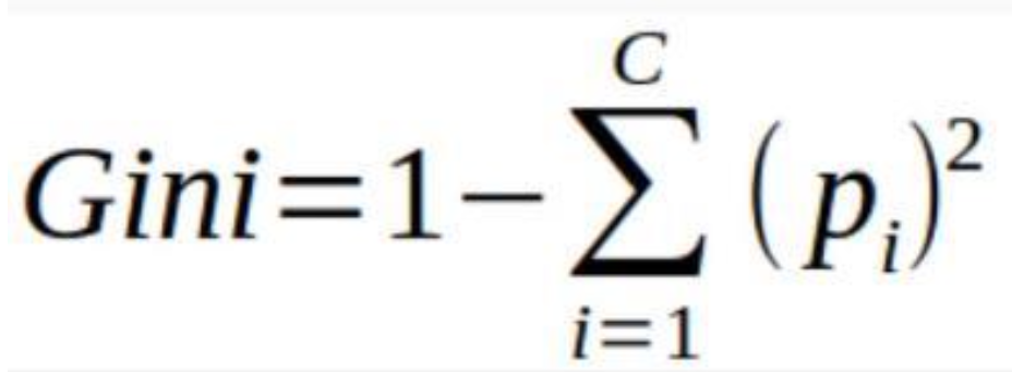
- Gini Index:
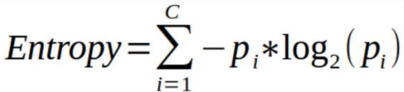
- Entropy:
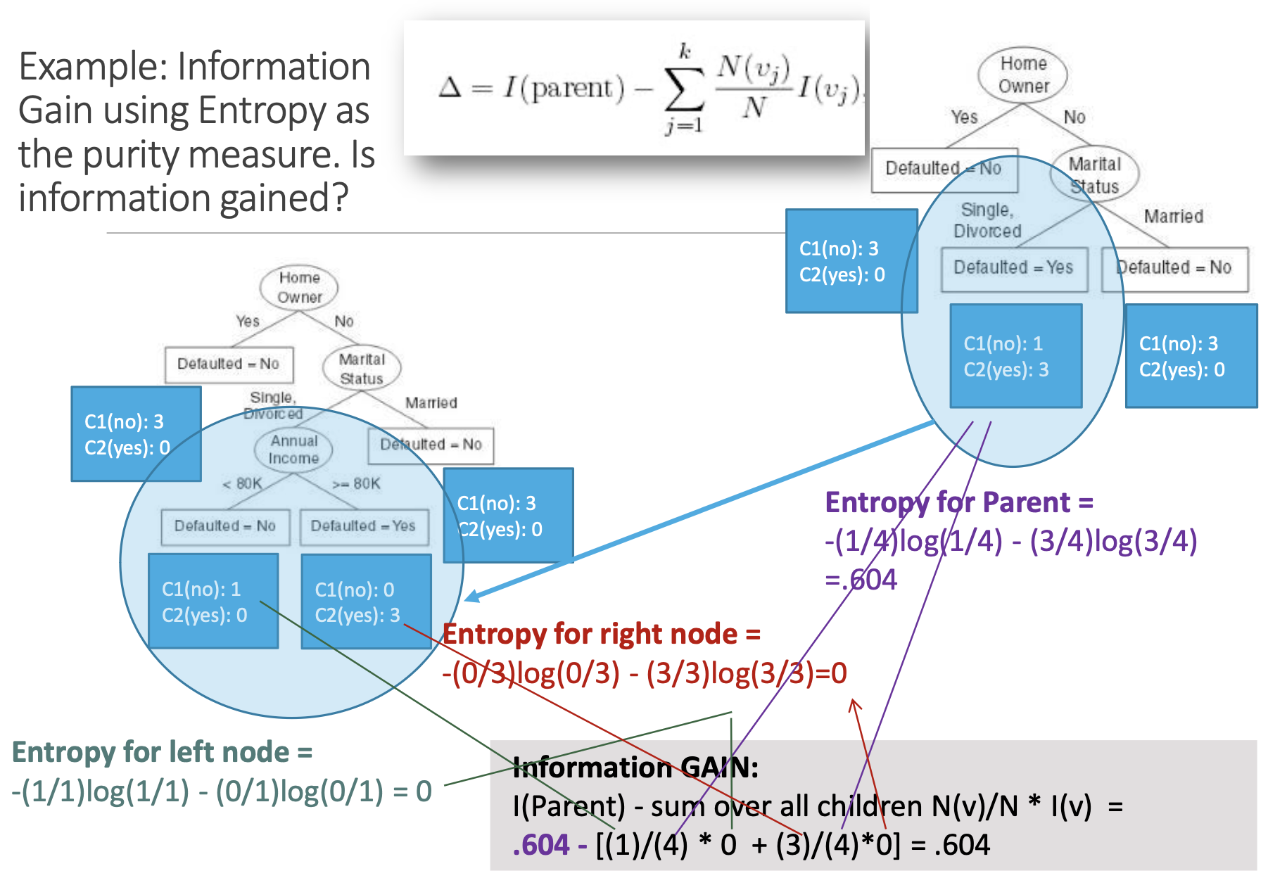
- Information Gain:
It measures the probability for a random instance being misclassified when choosen randomly. It ranges from 0 (pure node) to 0.5 (maximum impurity).
It measures the uncertainity or impurity in a node. It is calculated using the probability distribution of the classes in the node. Entropy ranges from 0 (pure node) to 1 (maximum impurity).
It is used to determine the strength of a partition i.e., to compare purity of parent node (before split) to child nodes (after split). Mathematically it is measure of the difference between impurity values before splitting the data at a node and the weighted average of the impurity after the split.The greater the difference – the better the partition condition.
The Gain (∆) is a measure for goodness of split.
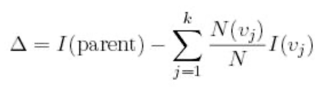
where,
I is the impurity measure of a node (such as GINI or Entropy)
N is the number of records/vectors/rows at parent node
k is the number of attribute values (variable options)
N(vj) is the number of records in child vj.
Depending on which impurity measurement is used, tree classification results can vary. There is no one preferred approach by different Decision Tree algorithms.
Example: CART uses Gini; ID3 and C4.5 use Entropy.
Calculation:
PLAN
- Load the cleaned Denver weather dataset, preprocess it to label weather descriptions, convert features into Category/Factor type, and filter data for Denver only.
- Split the dataset into training and testing sets using stratified sampling stratified sampling in python and random sampling without replacement in R to ensure proportional representation of each class in both sets.
- Train Decision Tree Classifier models with different criteria and splitter combinations, evaluate accuracy, and generate confusion matrices.
- Visualize the decision trees and plot their confusion matrices.
- Analyze feature importance to understand which features are most relevant for weather prediction.
DATA PREPARATION
R(rpart) can perform Decision Tree on mixed labeled data (quantitative and qualitative) whereas in Python (Sklearn), data must be quantitative and labeled.
- In sklearn, for classification tasks (DecisionTreeClassifier), the default criterion is 'gini', which refers to the Gini impurity.
- In sklearn, for regression tasks (DecisionTreeRegressor), the default criterion is 'mse', which stands for Mean Squared Error.
- In rpart, the default splitting criterion for regression trees is "ANOVA" (analysis of variance), while for classification trees, it's "gini" or "information gain" (using the deviance).
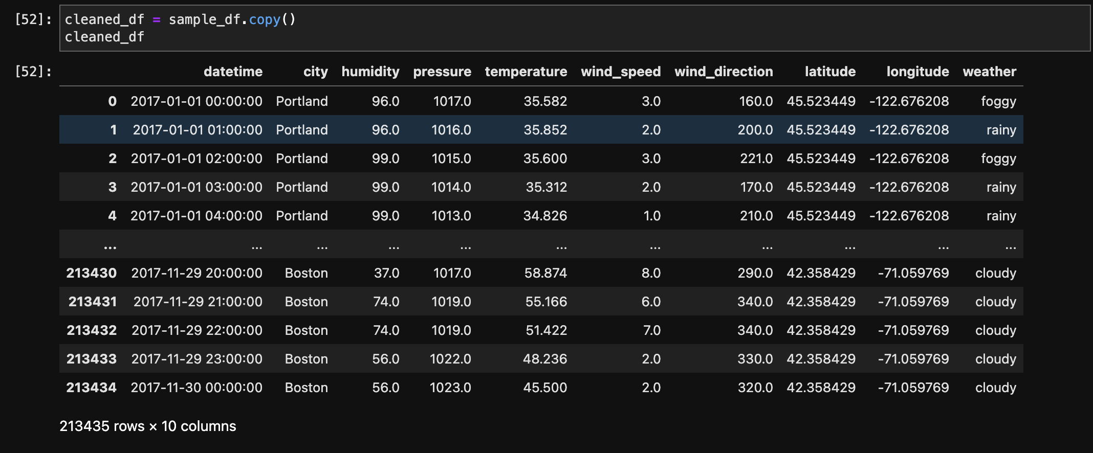
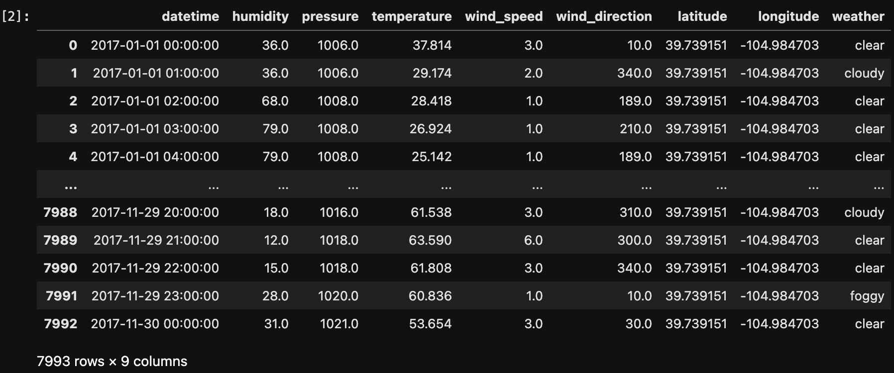
- Before Transformation:
- After Filtering Denver Data:
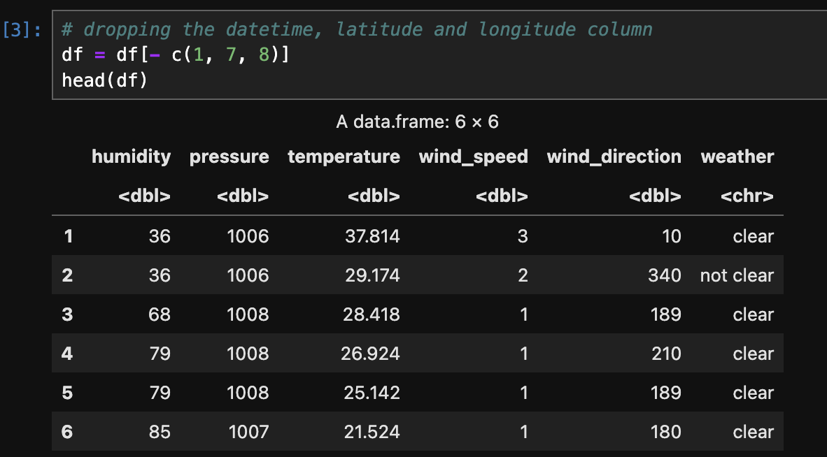
- After Transformation (Python):
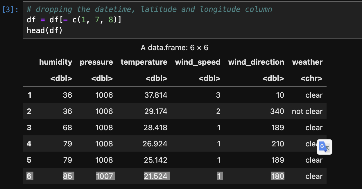
- After Transformation (R):
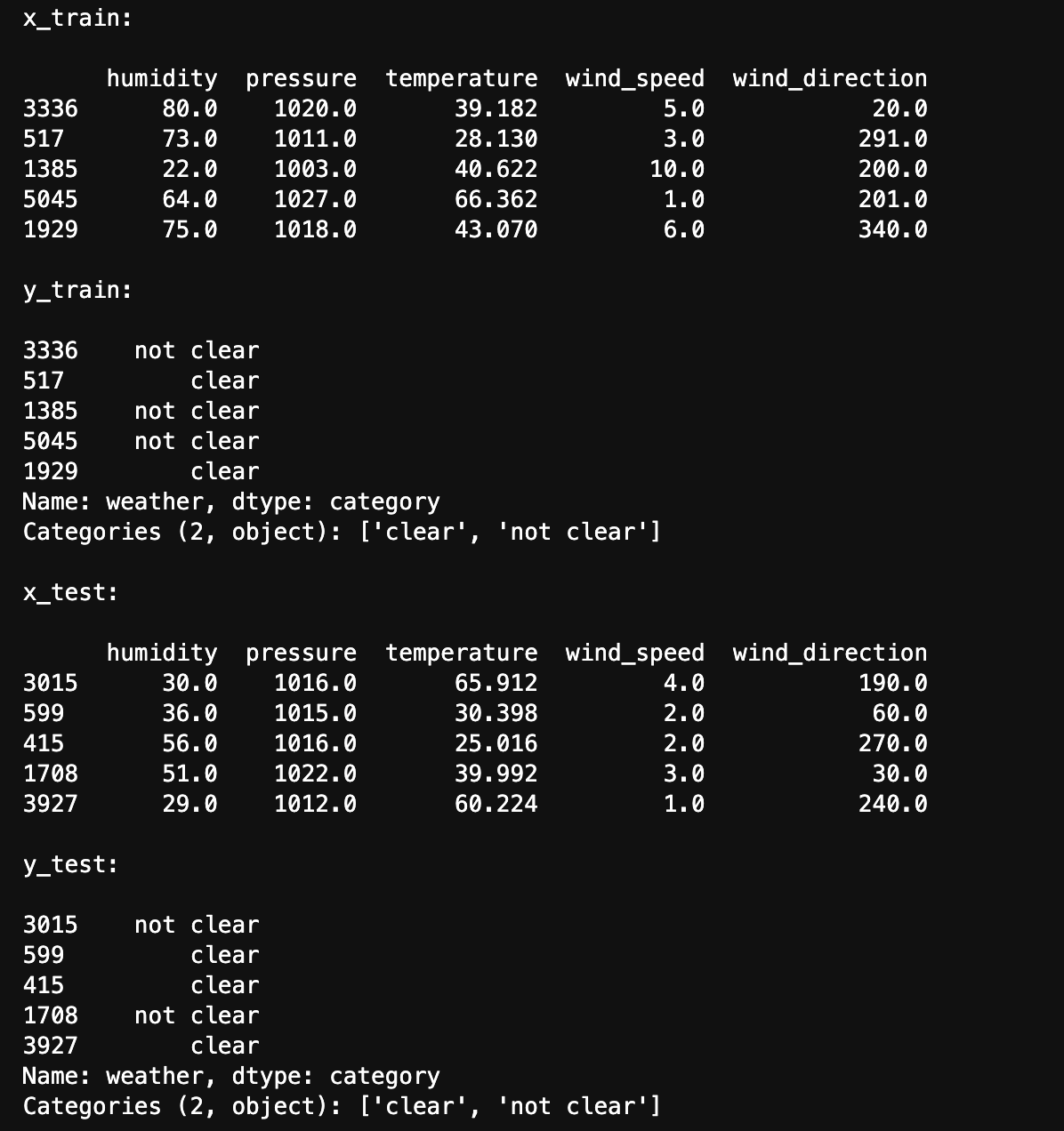
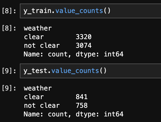
- Splitting data into Train and Test set (Python):
- Checking the balance of the Train and Test set (Python):
- Splitting data into Train and Test set (R):
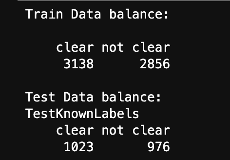
- Checking the balance of the Train and Test set (R):
- Classification Dataset:
The below image shows the sample of data before transformation.
The below image shows the data after filtering city by Denver.
The below image shows the data after after After labelling (clear/not clear) the data for classification and changing its type to Category.
The below image shows the labelling (clear/not clear) the data for classification and changing its type to Factor.
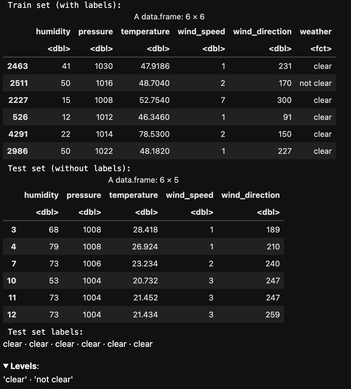
The below image shows train and test data created using stratified sampling to ensure that each class is represented proportionally in both sets. Train and test sets are disjoint to ensure that the model is evaluated on data it hasn't seen during training, enabling an unbiased assessment of its performance.
The below image shows the distribution of labels in the Train and Test set. They are well balanced.
The below image shows train and test data created using Random sample without replacement. Train and test sets are disjoint to ensure that the model is evaluated on data it hasn't seen during training, enabling an unbiased assessment of its performance.
The below image shows the distribution of labels in the Train and Test set. They are well balanced.
CODE
- Decision Tree (Python):
- Decision Tree (R):
RESULTS
- Accuracy (Python):
- Confusion Matrix (Python):
- Tree Viz. (Python):
- entropy criterion and best splitter:
- entropy criterion and random splitter:
- gini criterion and best splitter:
- gini criterion and random splitter:
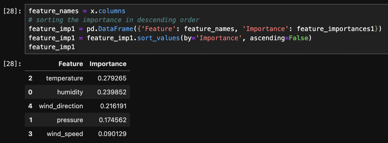
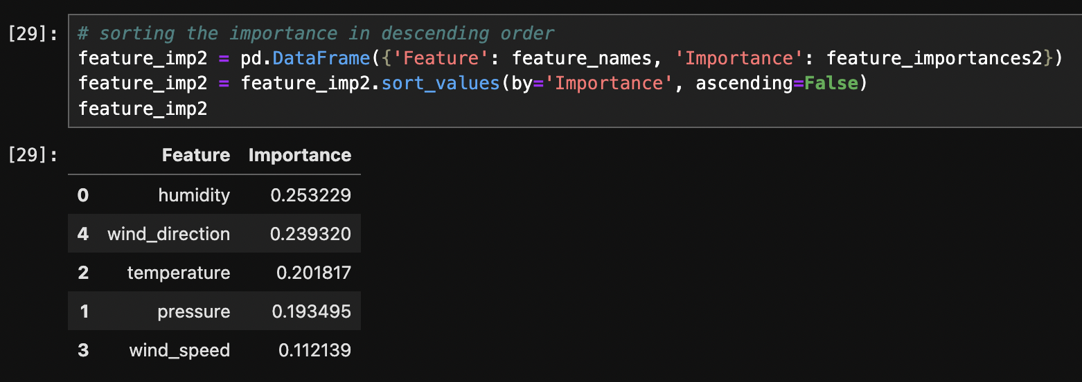
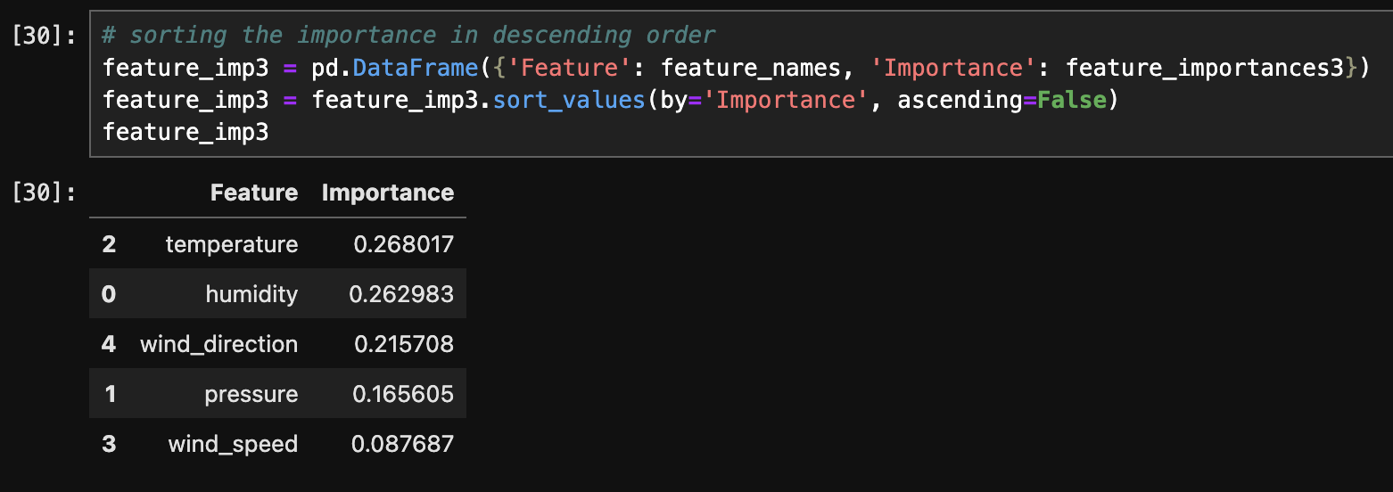
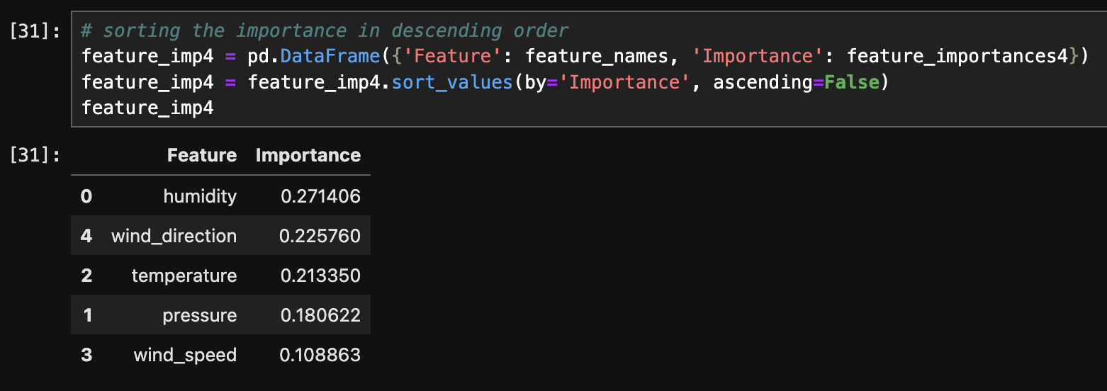
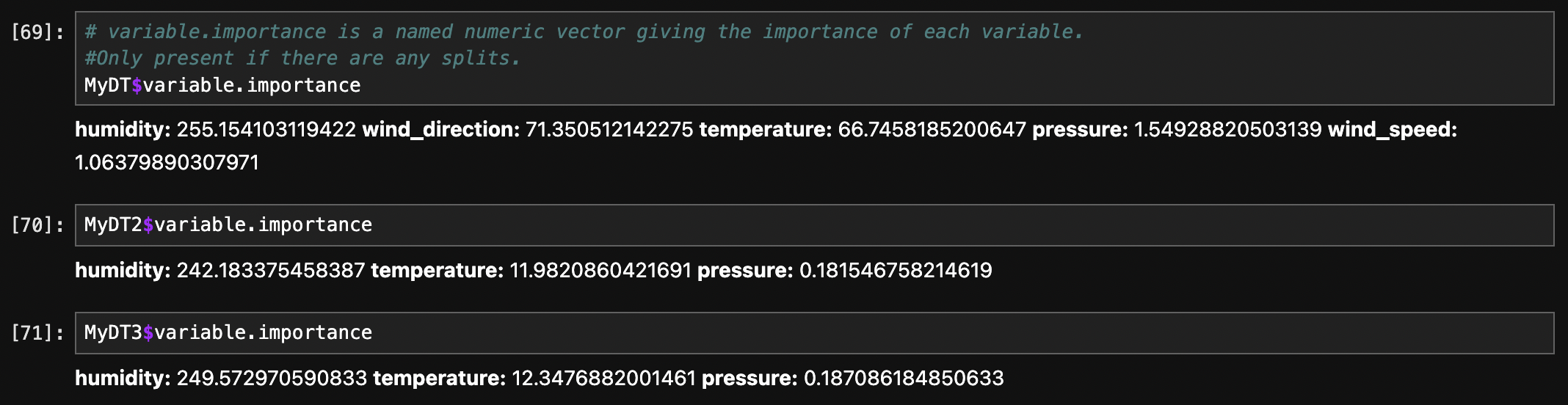
- Feature Importance (Python):
- CP plot (R):
- Accuracy and Confusion Matrix (R):
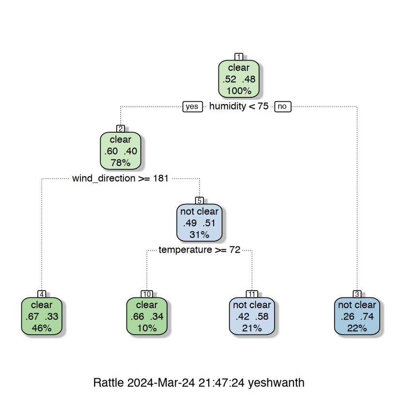
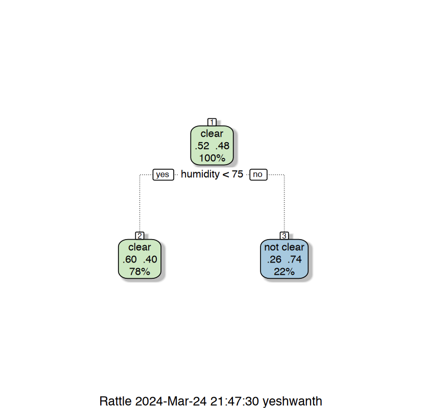
- Tree Viz. (R):
- Feature Importance (R):
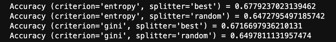
The above image displays accuracy of 4 different trees. Decision Tree with entropy criterion and best splitter achieved highest accuracy of 67.79%.
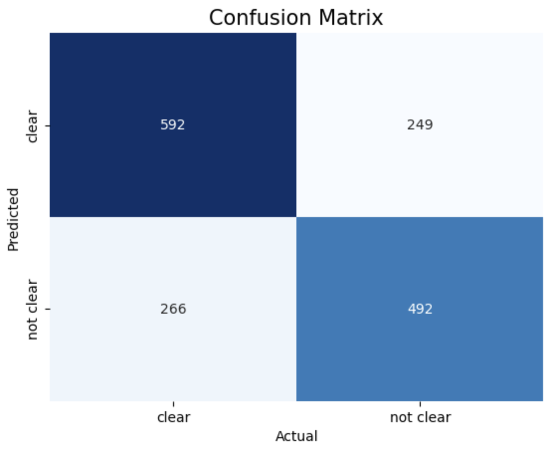
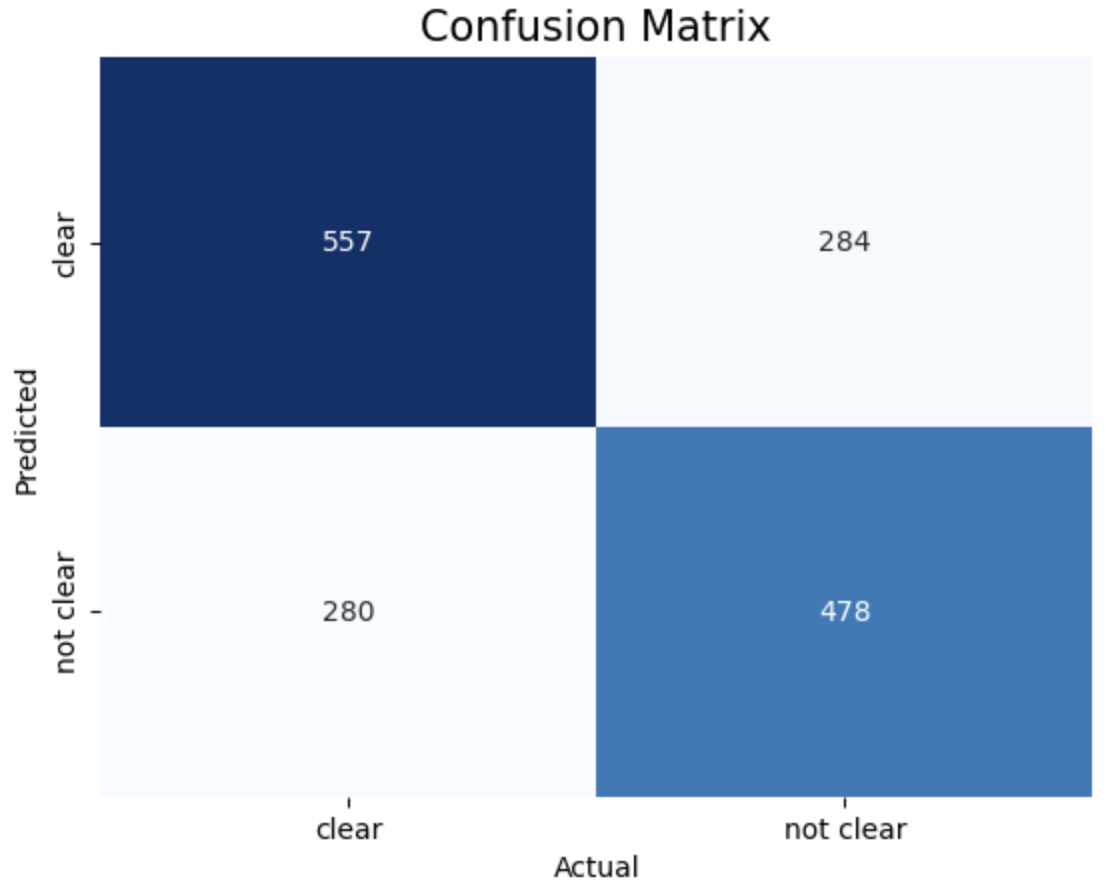
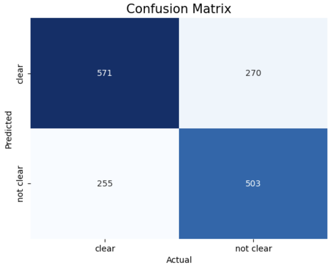
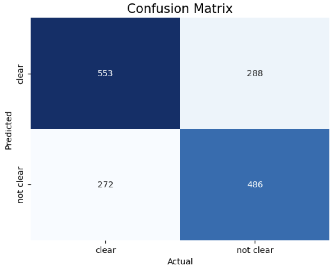
1. entropy criterion and best splitter 2. entropy criterion and random splitter 3. gini criterion and best splitter 4. gini criterion and random splitter.
The above images displays confusion matrix of 4 different trees.
The below links are the Tree visualization for 4 different trees.
1. entropy criterion and best splitter 2. entropy criterion and random splitter 3. gini criterion and best splitter 4. gini criterion and random splitter.
The above images displays the feature importance for each tree.
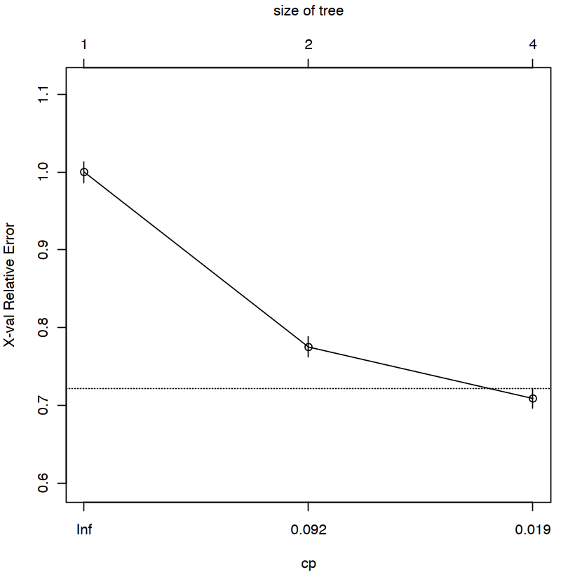
The above image displays CP plot.
The x-axis represents the complexity parameter (CP) values. Each point on the x-axis corresponds to a particular level of complexity parameter.
The y-axis represents the cross-validated error rate associated with each complexity parameter value.
The goal is to choose a CP value that results in a decision tree model with sufficient pruning to avoid overfitting, while still retaining good predictive performance on new data.
The small cp the larger the tree if cp is too small you have overfitting. So, choosing cp as 0.092
Where,
CP: Complexity parameter values.
nsplit: Number of splits in the tree.
rel error: It is the error rate relative to the root node (1.000 represents the error rate at the root node).
xerror:It is the Cross-validated error rate, which estimates the error rate of the tree on unseen data using cross-validation.
xstd: Standard error of the cross-validated error rate.
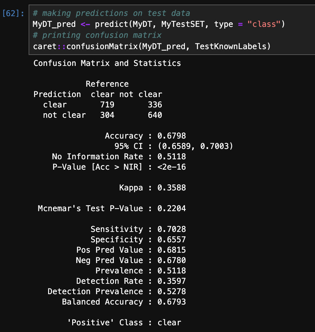
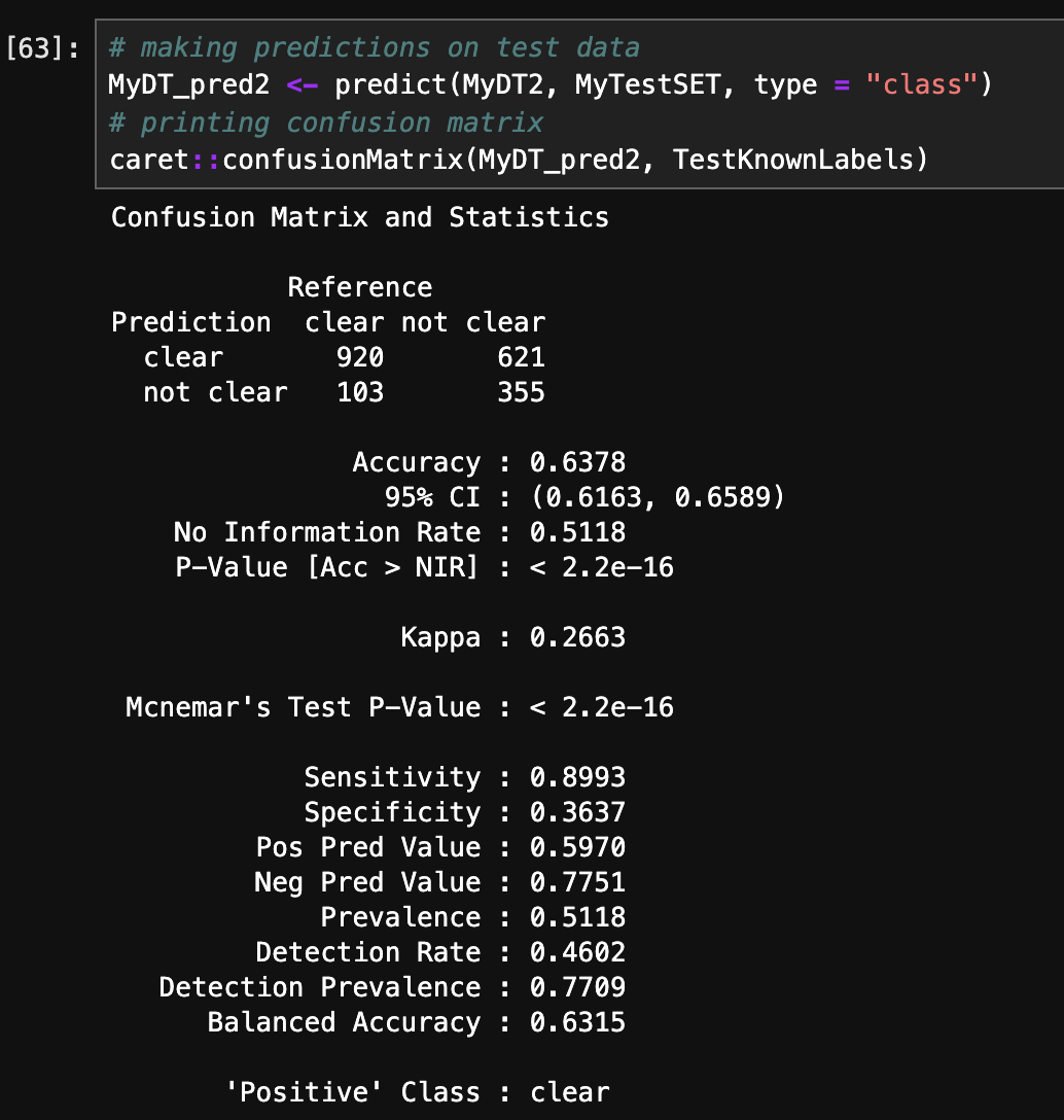
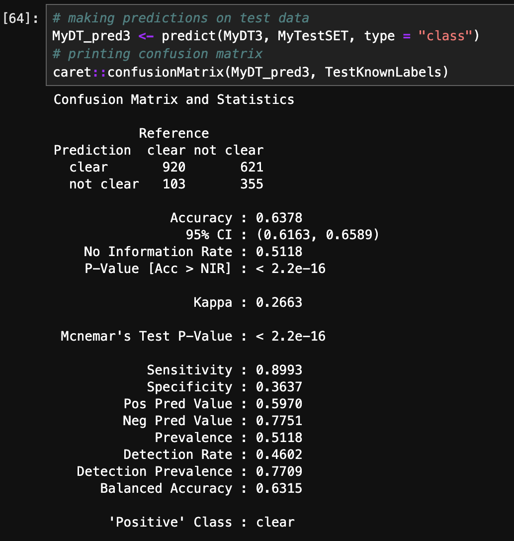
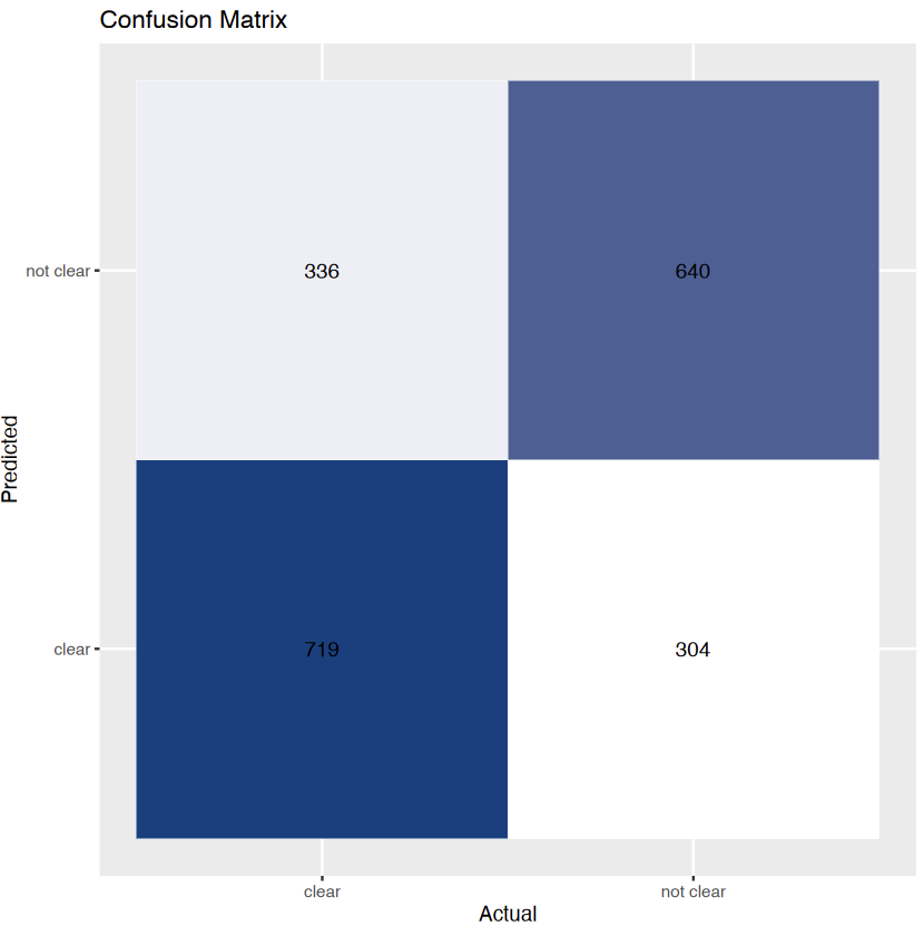
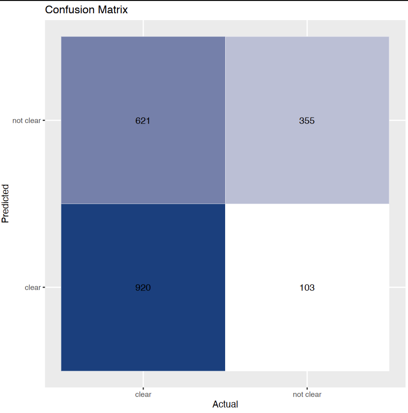
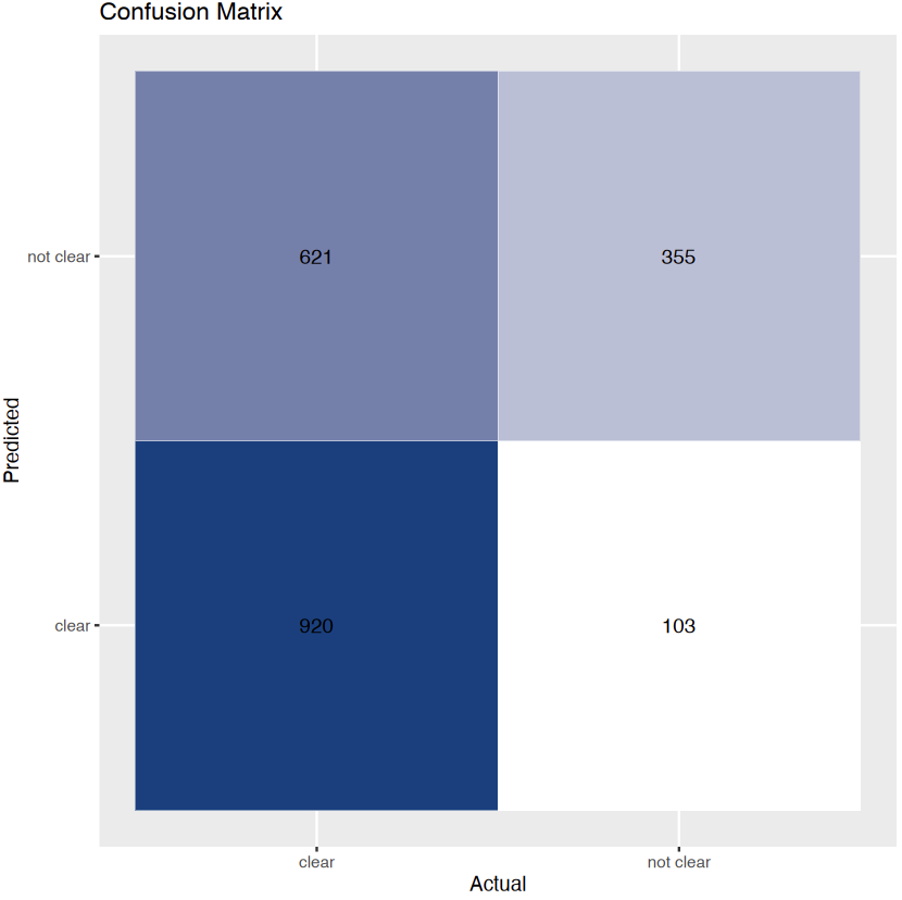
1. Decision tree with gini criterion (defualt) 2. Decision tree with gini criterion (defualt) and cp = 0.092 3. Decision tree with entropy criterion and cp = 0.092.
The above images displays accuracy and confusion matrix of 3 different trees. Decision Tree with gini criterion has achieved highest accuracy of 67.98%.

1. Decision tree with gini criterion (defualt) 2. Decision tree with gini criterion (defualt) and cp = 0.092 3. Decision tree with entropy criterion and cp = 0.092.
The above images are the Tree visualization for 3 different trees. The small cp the larger the tree if cp is too small you have overfitting.
1. Decision tree with gini criterion (default) 2. Decision tree with gini criterion (defualt) and cp = 0.092 3. Decision tree with entropy criterion and cp = 0.092.
The above images displays the feature importance for each tree.
CONCLUSION
This study focuses on clear weather prediction in Denver and its practical consequences for daily life. Understanding when the weather will clear is critical for a wide range of activities. From organizing outside gatherings like picnics and sports games to scheduling building projects and outdoor maintenance jobs. Clear weather also plays an important role in trip planning because it provides safer driving conditions and easier flights. Individuals and organizations can make better informed decisions by properly anticipating clear weather. It results in more efficient and enjoyable experiences in both personal and professional settings. The study's overall findings demonstrate the value of predictive modeling in precisely predicting clear weather, which eventually improves community well-being and resistance to weather-related issues. Through the utilization of these insights, individuals and organizations can enhance their decision-making abilities and guarantee safer and more pleasurable experiences for all stakeholders. Communities may improve their quality of life and resistance to weather-related changes by better understanding and preparing for weather-related concerns. This will create safer, more lively, and more sustainable settings for both locals and visitors.