SUPPORT VECTOR MACHINE
OVERVIEW
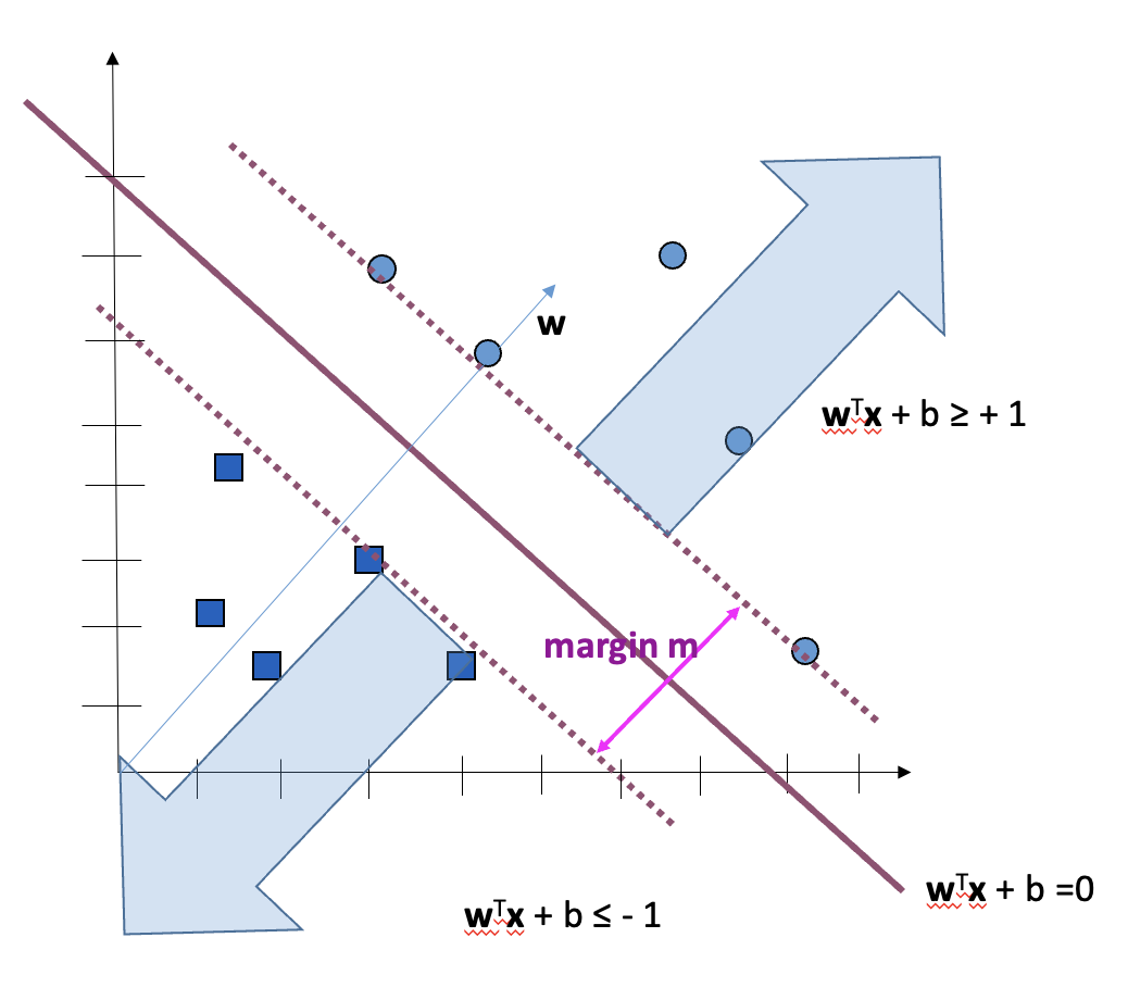
Support Vector Machines are a popular supervised learning algorithm used for both classification and regression tasks in machine learning.
They are linear separators as them find a linear decision boundary that separates the data points into different classes. This decision boundary is defined by a hyperplane in the feature space. It can only separate two categories. For multiple categories, at least 2 SVM's are required.
Kernel:
SVMs use Kernel which enables it to separate data which is not linearly separable in its dimensional space and finds a dimensional space where it is linearly seperable.
Suppose we have a function:
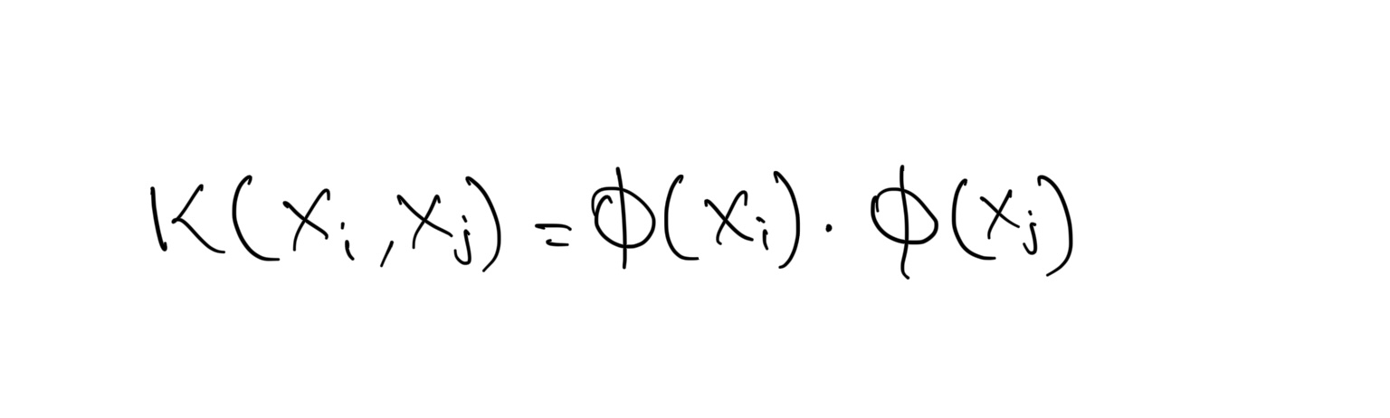
K is called a Kernel function. The Kernel function provides the dot product in another space.
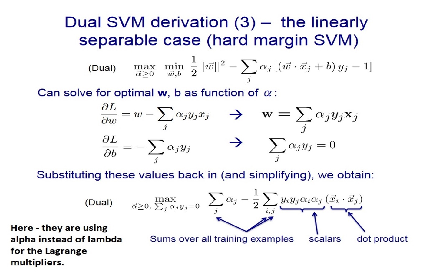
If we have n points in our dataset, the SVM needs only the dot product of each pair of points to find a classifier. This is also true when we want to project data to higher dimensions. We don’t need to provide the SVM with exact projections; we only need to give it the dot product between all pairs of points in the projected space. This is relevant because this is exactly what kernels do. A kernel, short for kernel function, takes as input two points in the original space, and directly gives us the dot product in the projected space.
- L as well as the decision boundary equation only depend on the dot products of vectors.
- Therefore, to optimize, we only need φ(xi) dot φ(xj) for all xk and for any kernel, φ
- For the decision boundary, all we need is: φ(xi) dot (φ(xnew)) for any kernel φ. Therefore – we only need dot products.
There are different types of Kernels.
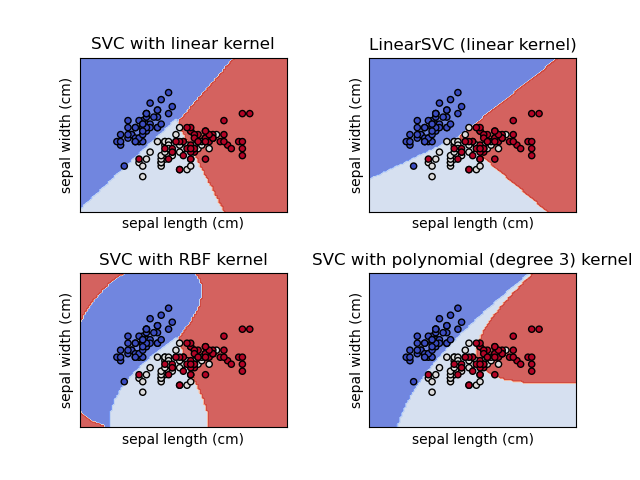
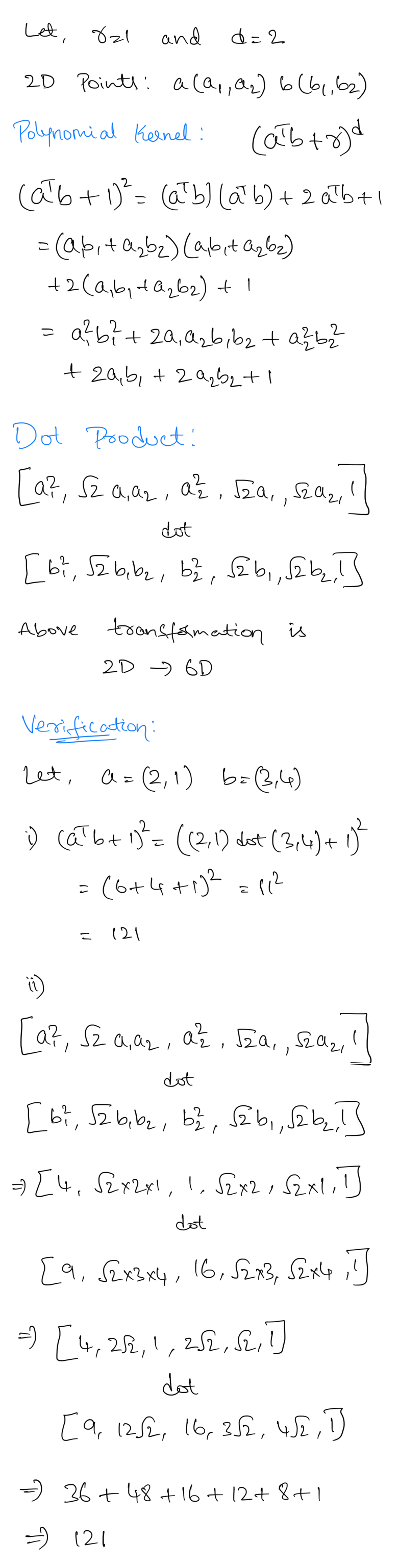
Polynomial Kernel:
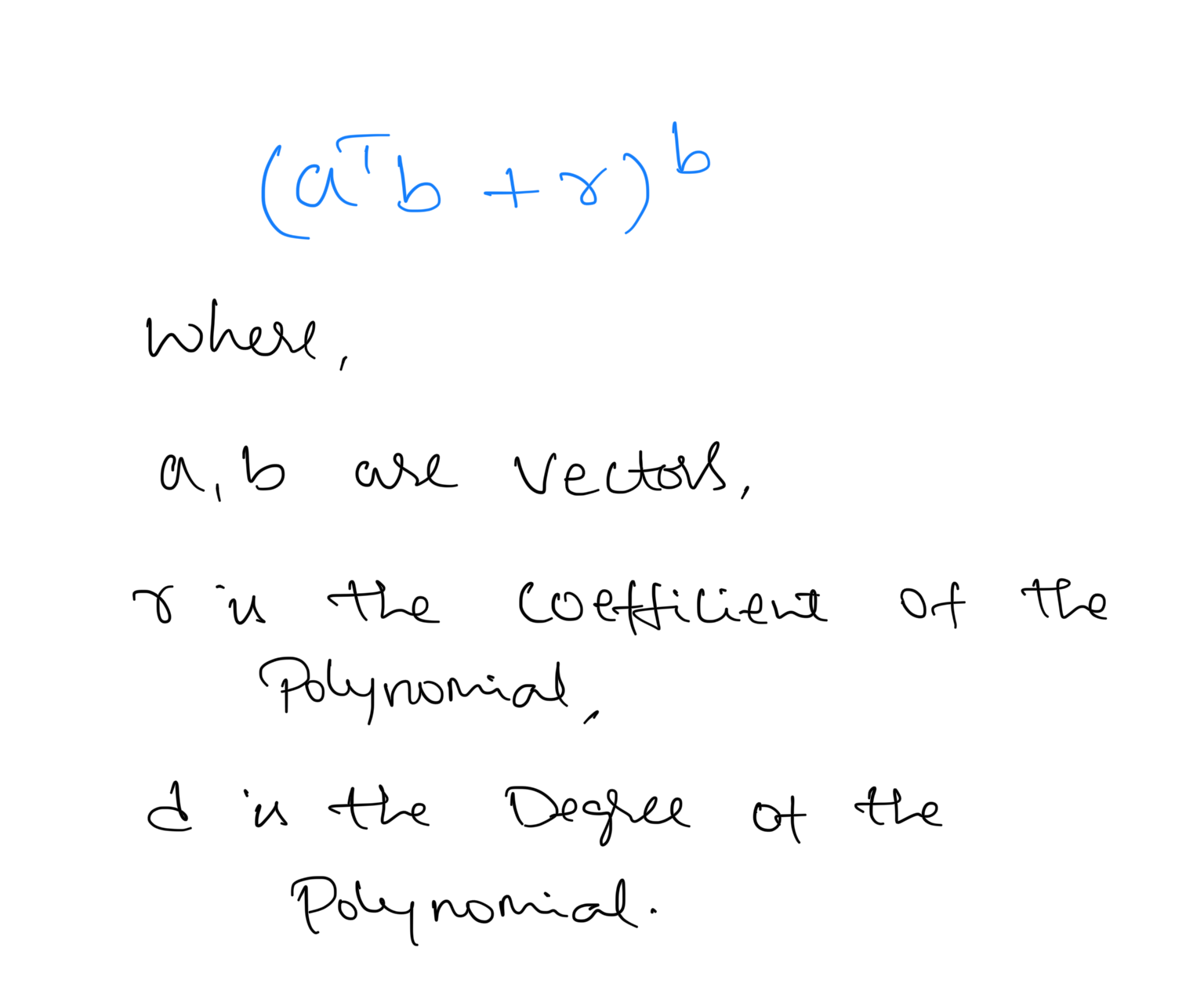
Example:
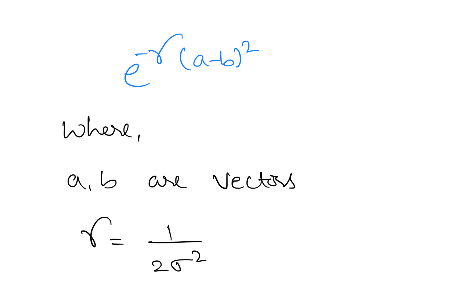
RBF (Radial Basis Function) Kernel:
PLAN
- Load the cleaned Denver weather dataset, preprocess it to label weather descriptions, convert features into Category/Factor type, and filter data for Denver only.
- Split the dataset into training and testing sets using stratified sampling stratified sampling in python and random sampling without replacement in R to ensure proportional representation of each class in both sets.
- Train SVM Classifier models with different kernels and cost combinations, evaluate accuracy, and generate confusion matrices.
DATA PREPARATION
- SVM require labeled data for training.
- SVMs specifically require numerical (Quantitative) data because they rely on mathematical computations to find the optimal hyperplane that best separates the different classes in the feature space. This hyperplane is determined by maximizing the margin between the classes, which involves calculating distances and dot products between data points.
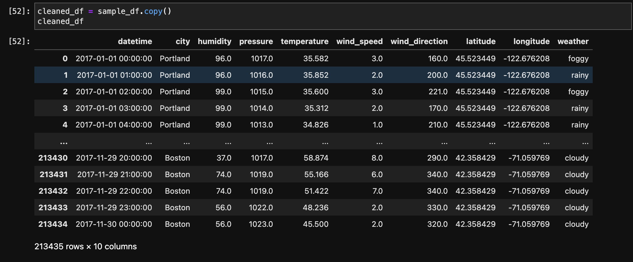
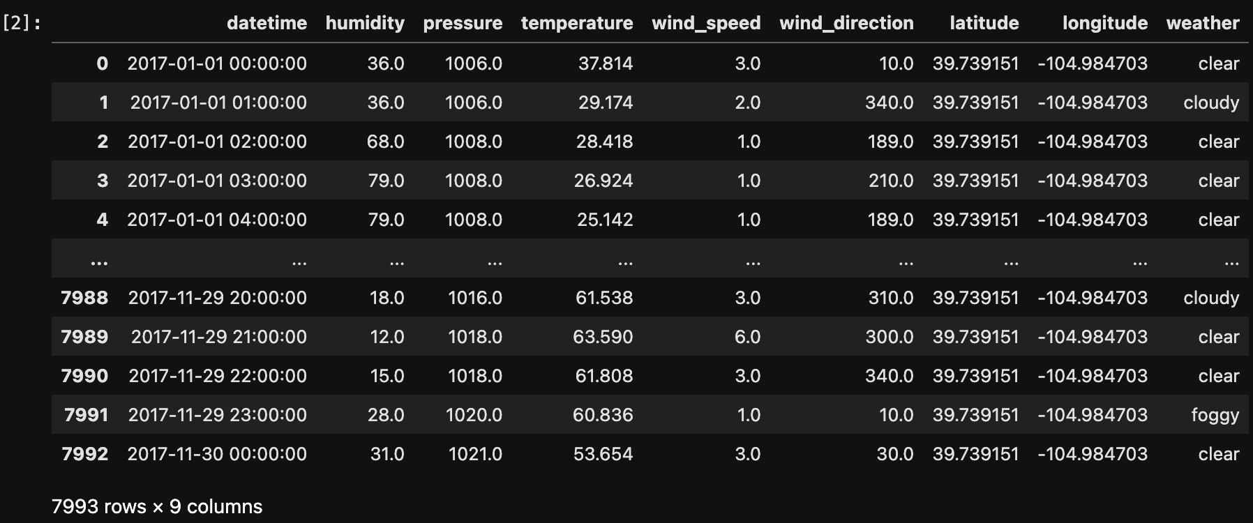
- Before Transformation:
- After Filtering Denver Data:
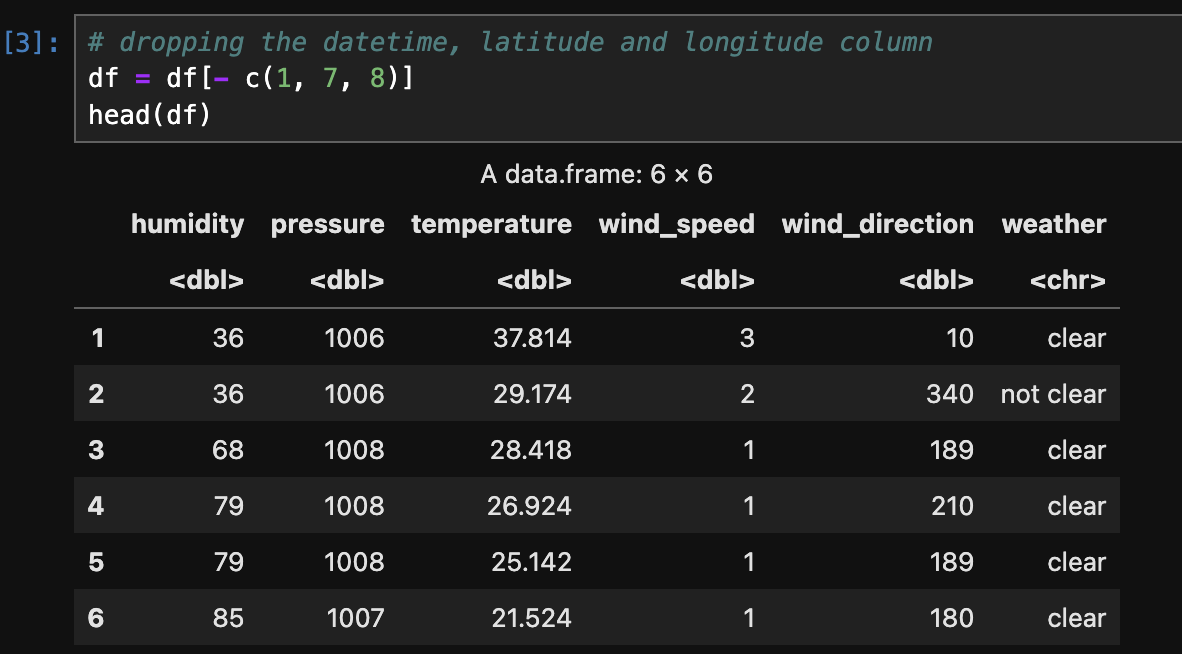
- After Transformation (Python):
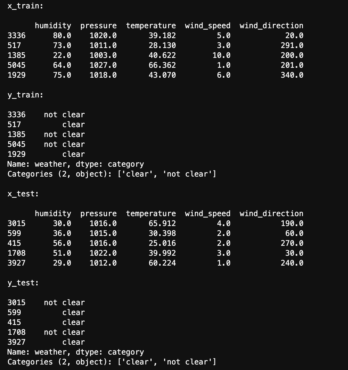
- Splitting data into Train and Test set (Python):
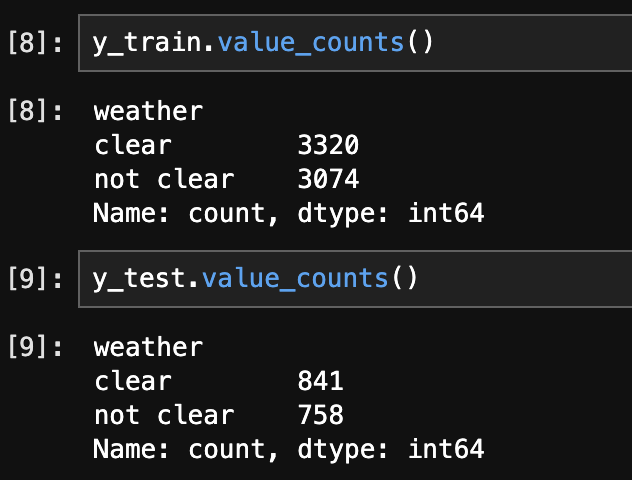
- Checking the balance of the Train and Test set (Python):
- Classification Dataset:
The below image shows the sample of data before transformation.
The below image shows the data after filtering city by Denver.
The below image shows the data after after After labelling (clear/not clear) the data for classification and changing its type to Category.
The below image shows train and test data created using stratified sampling to ensure that each class is represented proportionally in both sets. Train and test sets are disjoint to ensure that the model is evaluated on data it hasn't seen during training, enabling an unbiased assessment of its performance.
The below image shows the distribution of labels in the Train and Test set. They are well balanced.
CODE
- SVM (Python):
RESULTS
- Accuracy:
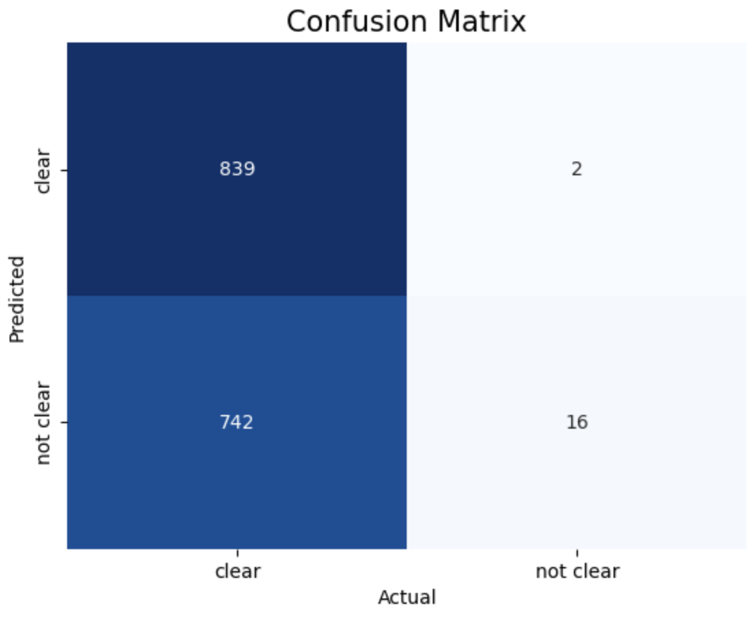
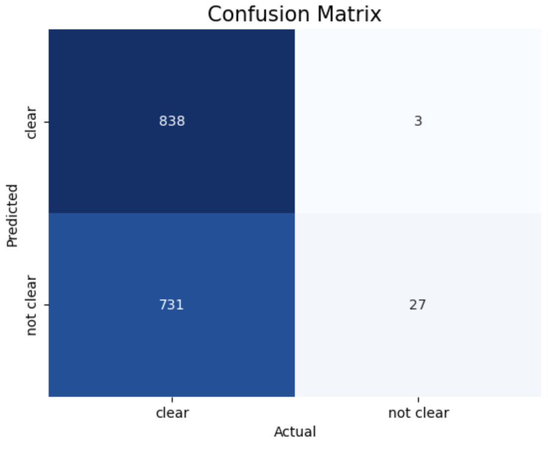
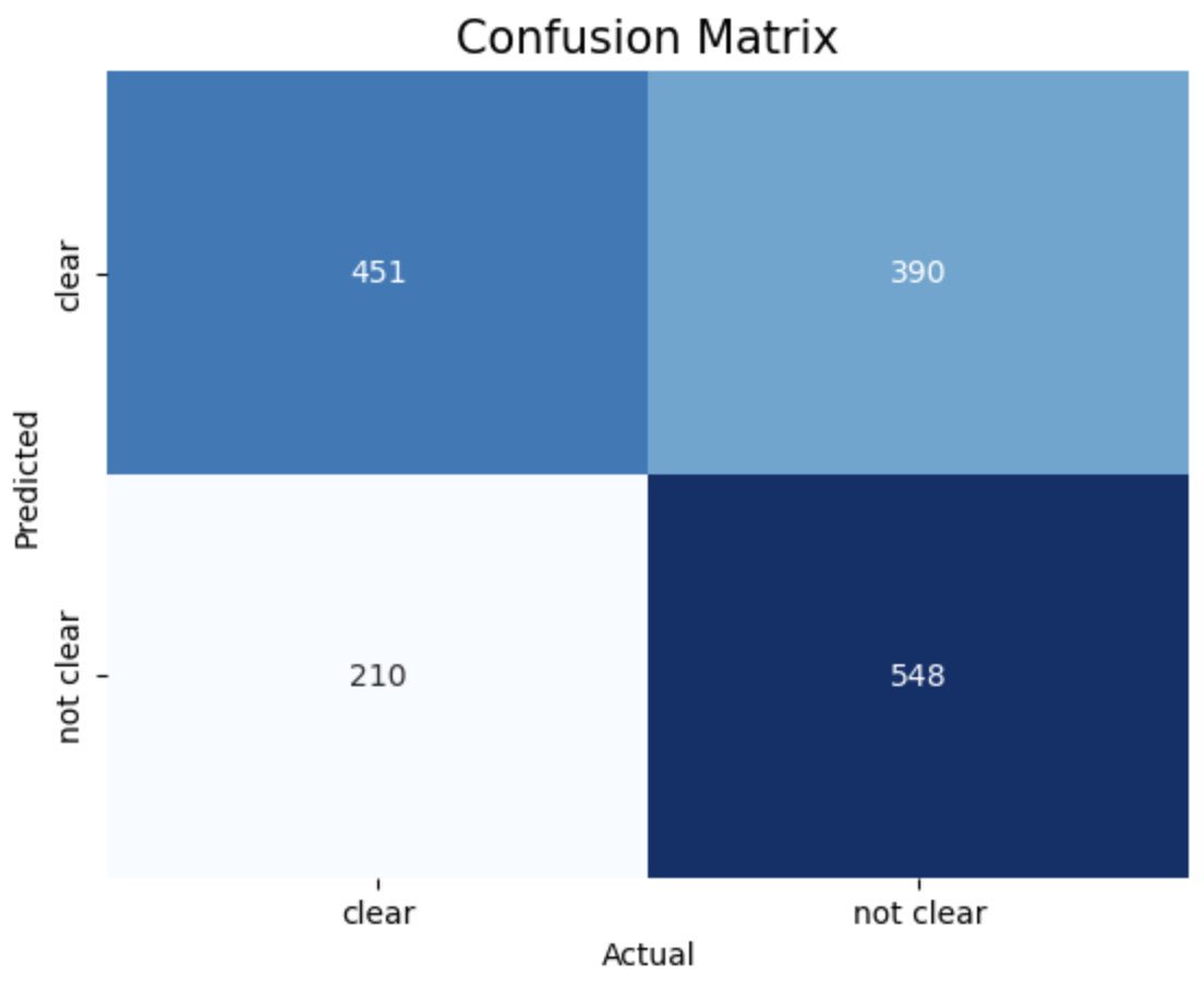
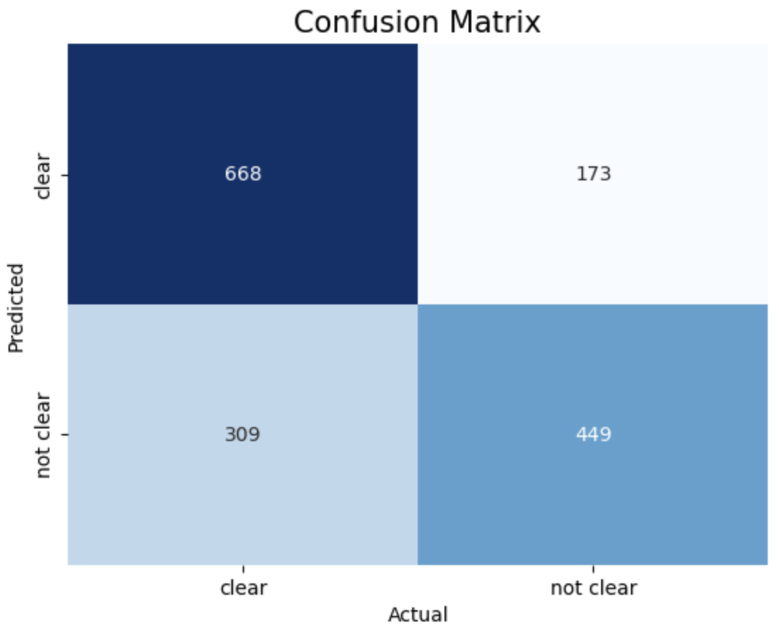
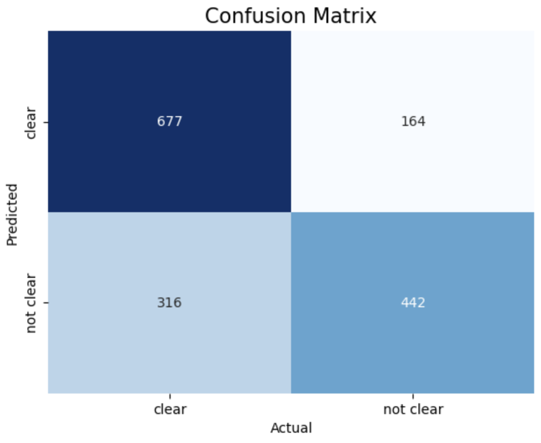
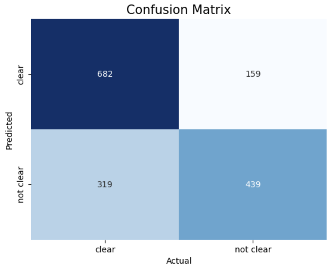
- Confusion Matrix:
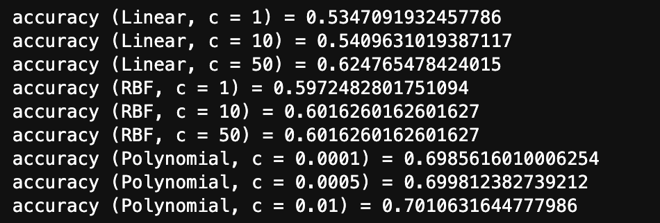
The provided results show the accuracy scores of Support Vector Machine (SVM) models trained with different kernels (linear, RBF, polynomial) and different values of the cost function 𝐶.
SVM model with Polynomial Kernel and Cost function achieved highest accuracy of 70.1%
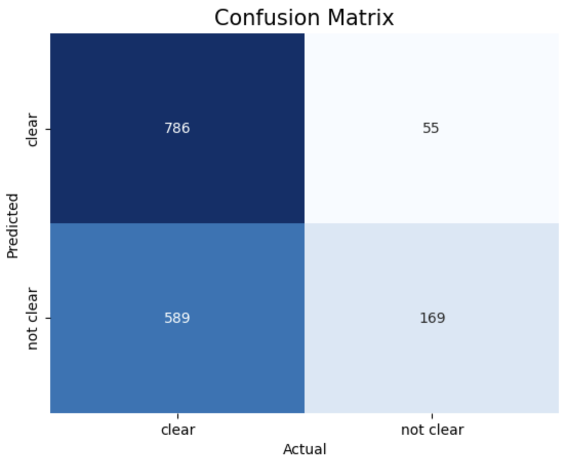


1. Linear, c = 1 2. Linear, c = 10 3. Linear, c = 50
4. RBF, c = 1 5. RBF, c = 10 6. RBF, c = 50
7. Polynomial, c = 0.0001 8. Polynomial, c = 0.0005 9. Polynomial, c = 0.001
The above images displays confusion matrix of 8 different SVM models trained with different Kernel and Cost function.
CONCLUSION
This study focuses on clear weather prediction in Denver and its practical consequences for daily life. Understanding when the weather will clear is critical for a wide range of activities. From organizing outside gatherings like picnics and sports games to scheduling building projects and outdoor maintenance jobs. Clear weather also plays an important role in trip planning because it provides safer driving conditions and easier flights. Individuals and organizations can make better informed decisions by properly anticipating clear weather. It results in more efficient and enjoyable experiences in both personal and professional settings. The study's overall findings demonstrate the value of predictive modeling in precisely predicting clear weather, which eventually improves community well-being and resistance to weather-related issues. Through the utilization of these insights, individuals and organizations can enhance their decision-making abilities and guarantee safer and more pleasurable experiences for all stakeholders. Communities may improve their quality of life and resistance to weather-related changes by better understanding and preparing for weather-related concerns. This will create safer, more lively, and more sustainable settings for both locals and visitors.